Usage

This usage tutorial shows how to fit historical control-group borrowing models using the historicalborrowlong package.

Data

historicalborrowlong expects data on multiple patients partitioned into studies, groups, and repeated measures (“reps”). Here is a simulated example. There are functions to simulate from the prior predictive distribution of each of the hierarchical, independent, and pooled models.

library(historicalborrowlong)
library(dplyr)
set.seed(0)
data <- hbl_sim_independent(
  n_continuous = 1,
  n_study = 3,
  n_group = 2,
  n_rep = 4,
  alpha = rep(1, 12),
  delta = rep(0.5, 4),
  n_patient = 10
)$data %>%
  rename(
    outcome = response,
    trial = study,
    arm = group,
    subject = patient,
    visit = rep,
    factor1 = covariate_study1_continuous1,
    factor2 = covariate_study2_continuous1
  ) %>%
  mutate(
    trial = paste0("trial", trial),
    arm = paste0("arm", arm),
    subject = paste0("subject", subject),
    visit = paste0("visit", visit),
  )
data
#> # A tibble: 160 × 8
#>    trial  arm   subject  visit  factor1 factor2 covariate_study3_conti…¹ outcome
#>    <chr>  <chr> <chr>    <chr>    <dbl>   <dbl>                    <dbl>   <dbl>
#>  1 trial1 arm1  subject1 visit1   0.764       0                        0  2.82  
#>  2 trial1 arm1  subject1 visit2   0.764       0                        0  3.40  
#>  3 trial1 arm1  subject1 visit3   0.764       0                        0  3.30  
#>  4 trial1 arm1  subject1 visit4   0.764       0                        0  3.02  
#>  5 trial1 arm1  subject2 visit1  -0.799       0                        0 -0.504 
#>  6 trial1 arm1  subject2 visit2  -0.799       0                        0  0.0952
#>  7 trial1 arm1  subject2 visit3  -0.799       0                        0  0.441 
#>  8 trial1 arm1  subject2 visit4  -0.799       0                        0 -0.0921
#>  9 trial1 arm1  subject3 visit1  -1.15        0                        0 -0.0738
#> 10 trial1 arm1  subject3 visit2  -1.15        0                        0 -1.13  
#> # ℹ 150 more rows
#> # ℹ abbreviated name: ¹covariate_study3_continuous1

You as the user will choose a reference level of the study (“trial”) column to indicate which study is the current one (the other are historical). Likewise, you will choose a level of the group (“arm”) column to indicate which group is the control group and a level of the rep (“visit”) column to indicate the first measurement of each patient (baseline). To see how historicalborrowlong assigns numeric indexes to the study and group levels, use hbl_data(). Viewing this output may assist with interpreting the results later on.

standardized_data <- hbl_data(
  data = data,
  response = "outcome",
  study = "trial",
  study_reference = "trial3",
  group = "arm",
  group_reference = "arm1",
  patient = "subject",
  rep = "visit",
  rep_reference = "visit1",
  # Can be continuous, categorical, or binary columns:
  covariates = c("factor1", "factor2")
)
standardized_data
#> # A tibble: 160 × 11
#>    study patient patient_label   rep rep_label response study_label group_label
#>    <int>   <int> <chr>         <int> <chr>        <dbl> <chr>       <chr>      
#>  1     1       1 subject1          1 visit1      2.82   trial1      arm1       
#>  2     1       1 subject1          2 visit2      3.40   trial1      arm1       
#>  3     1       1 subject1          3 visit3      3.30   trial1      arm1       
#>  4     1       1 subject1          4 visit4      3.02   trial1      arm1       
#>  5     1       2 subject10         1 visit1      0.343  trial1      arm1       
#>  6     1       2 subject10         2 visit2     -1.46   trial1      arm1       
#>  7     1       2 subject10         3 visit3     -0.747  trial1      arm1       
#>  8     1       2 subject10         4 visit4      0.155  trial1      arm1       
#>  9     1      12 subject2          1 visit1     -0.504  trial1      arm1       
#> 10     1      12 subject2          2 visit2      0.0952 trial1      arm1       
#> # ℹ 150 more rows
#> # ℹ 3 more variables: group <int>, covariate_factor1 <dbl>,
#> #   covariate_factor2 <dbl>

distinct(
  standardized_data,
  study,
  study_label,
  group,
  group_label,
  rep,
  rep_label
) %>%
  select(
    study,
    study_label,
    group,
    group_label,
    rep,
    rep_label
  )
#> # A tibble: 16 × 6
#>    study study_label group group_label   rep rep_label
#>    <int> <chr>       <int> <chr>       <int> <chr>    
#>  1     1 trial1          1 arm1            1 visit1   
#>  2     1 trial1          1 arm1            2 visit2   
#>  3     1 trial1          1 arm1            3 visit3   
#>  4     1 trial1          1 arm1            4 visit4   
#>  5     2 trial2          1 arm1            1 visit1   
#>  6     2 trial2          1 arm1            2 visit2   
#>  7     2 trial2          1 arm1            3 visit3   
#>  8     2 trial2          1 arm1            4 visit4   
#>  9     3 trial3          1 arm1            1 visit1   
#> 10     3 trial3          1 arm1            2 visit2   
#> 11     3 trial3          1 arm1            3 visit3   
#> 12     3 trial3          1 arm1            4 visit4   
#> 13     3 trial3          2 arm2            1 visit1   
#> 14     3 trial3          2 arm2            2 visit2   
#> 15     3 trial3          2 arm2            3 visit3   
#> 16     3 trial3          2 arm2            4 visit4

As explained in the hbl_data() and hbl_mcmc_*() help files, before running the MCMC, dataset is pre-processed. This includes expanding the rows of the data so every rep of every patient gets an explicit row. So if your original data has irregular rep IDs, e.g. unscheduled visits in a clinical trial that few patients attend, please remove them before the analysis. Only the most common rep IDs should be added.

After expanding the rows, the function fills in missing values for every column except the response. That includes covariates. Missing covariate values are filled in, first with last observation carried forward, then with last observation carried backward. If there are still missing values after this process, the program throws an informative error.

Models

Recommended: run all models using `hbl_mcmc_sge()`

The hbl_mcmc_sge() function runs all 3 models of interest on a Sun Grid Engine (SGE) computing cluster and returns a list of results from all three models. For standardized analyses of real studies, this is highly recommended over the alternative of running each model separately (hbl_mcmc_hierarchical(), hbl_mcmc_pool(), and hbl_mcmc_independent(), as in the next subsection).

In hbl_mcmc_sge(), each model runs in its own SGE job, and chains run in parallel across the cores available to each job. The return value is a list of results from each model (hierarchical, independent, and pooled) that you would get by running hbl_mcmc_hierarchical(), hbl_mcmc_pool(), and hbl_mcmc_independent() separately. Each of these data frames each be supplied separately to hbl_summary() as explained later in this vignette.

mcmc <- hbl_mcmc_sge(
  data = data,
  response = "outcome",
  study = "trial",
  study_reference = "trial3",
  group = "arm",
  group_reference = "arm1",
  patient = "subject",
  rep = "visit",
  rep_reference = "visit1",
  # Can be continuous, categorical, or binary columns:
  covariates = c("factor1", "factor2"),
  # Raise these arguments for serious analyses:
  chains = 1, # Increase to about 3 or 4 in real-life use cases.
  cores = 1, # *HIGHLY* recommended to have cores = chains
  iter = 20, # Increase to several thousand in real-life use cases.
  warmup = 10, # Increase to several thousand in real-life use cases.
  log = "/dev/null", # optional SGE log file, /dev/null to disregard the log
  scheduler = "local" # Set to "sge" for serious analysis.
)

#> 
#> SAMPLING FOR MODEL 'historicalborrowlong' NOW (CHAIN 1).
#> Chain 1: 
#> Chain 1: Gradient evaluation took 8.2e-05 seconds
#> Chain 1: 1000 transitions using 10 leapfrog steps per transition would take 0.82 seconds.
#> Chain 1: Adjust your expectations accordingly!
#> Chain 1: 
#> Chain 1: 
#> Chain 1: WARNING: No variance estimation is
#> Chain 1:          performed for num_warmup < 20
#> Chain 1: 
#> Chain 1: Iteration:  1 / 20 [  5%]  (Warmup)
#> Chain 1: Iteration:  2 / 20 [ 10%]  (Warmup)
#> Chain 1: Iteration:  4 / 20 [ 20%]  (Warmup)
#> Chain 1: Iteration:  6 / 20 [ 30%]  (Warmup)
#> Chain 1: Iteration:  8 / 20 [ 40%]  (Warmup)
#> Chain 1: Iteration: 10 / 20 [ 50%]  (Warmup)
#> Chain 1: Iteration: 11 / 20 [ 55%]  (Sampling)
#> Chain 1: Iteration: 12 / 20 [ 60%]  (Sampling)
#> Chain 1: Iteration: 14 / 20 [ 70%]  (Sampling)
#> Chain 1: Iteration: 16 / 20 [ 80%]  (Sampling)
#> Chain 1: Iteration: 18 / 20 [ 90%]  (Sampling)
#> Chain 1: Iteration: 20 / 20 [100%]  (Sampling)
#> Chain 1: 
#> Chain 1:  Elapsed Time: 0.413 seconds (Warm-up)
#> Chain 1:                0.571 seconds (Sampling)
#> Chain 1:                0.984 seconds (Total)
#> Chain 1: 
#> 
#> SAMPLING FOR MODEL 'historicalborrowlong' NOW (CHAIN 1).
#> Chain 1: 
#> Chain 1: Gradient evaluation took 6.8e-05 seconds
#> Chain 1: 1000 transitions using 10 leapfrog steps per transition would take 0.68 seconds.
#> Chain 1: Adjust your expectations accordingly!
#> Chain 1: 
#> Chain 1: 
#> Chain 1: WARNING: No variance estimation is
#> Chain 1:          performed for num_warmup < 20
#> Chain 1: 
#> Chain 1: Iteration:  1 / 20 [  5%]  (Warmup)
#> Chain 1: Iteration:  2 / 20 [ 10%]  (Warmup)
#> Chain 1: Iteration:  4 / 20 [ 20%]  (Warmup)
#> Chain 1: Iteration:  6 / 20 [ 30%]  (Warmup)
#> Chain 1: Iteration:  8 / 20 [ 40%]  (Warmup)
#> Chain 1: Iteration: 10 / 20 [ 50%]  (Warmup)
#> Chain 1: Iteration: 11 / 20 [ 55%]  (Sampling)
#> Chain 1: Iteration: 12 / 20 [ 60%]  (Sampling)
#> Chain 1: Iteration: 14 / 20 [ 70%]  (Sampling)
#> Chain 1: Iteration: 16 / 20 [ 80%]  (Sampling)
#> Chain 1: Iteration: 18 / 20 [ 90%]  (Sampling)
#> Chain 1: Iteration: 20 / 20 [100%]  (Sampling)
#> Chain 1: 
#> Chain 1:  Elapsed Time: 0.075 seconds (Warm-up)
#> Chain 1:                0.087 seconds (Sampling)
#> Chain 1:                0.162 seconds (Total)
#> Chain 1: 
#> 
#> SAMPLING FOR MODEL 'historicalborrowlong' NOW (CHAIN 1).
#> Chain 1: 
#> Chain 1: Gradient evaluation took 6.8e-05 seconds
#> Chain 1: 1000 transitions using 10 leapfrog steps per transition would take 0.68 seconds.
#> Chain 1: Adjust your expectations accordingly!
#> Chain 1: 
#> Chain 1: 
#> Chain 1: WARNING: No variance estimation is
#> Chain 1:          performed for num_warmup < 20
#> Chain 1: 
#> Chain 1: Iteration:  1 / 20 [  5%]  (Warmup)
#> Chain 1: Iteration:  2 / 20 [ 10%]  (Warmup)
#> Chain 1: Iteration:  4 / 20 [ 20%]  (Warmup)
#> Chain 1: Iteration:  6 / 20 [ 30%]  (Warmup)
#> Chain 1: Iteration:  8 / 20 [ 40%]  (Warmup)
#> Chain 1: Iteration: 10 / 20 [ 50%]  (Warmup)
#> Chain 1: Iteration: 11 / 20 [ 55%]  (Sampling)
#> Chain 1: Iteration: 12 / 20 [ 60%]  (Sampling)
#> Chain 1: Iteration: 14 / 20 [ 70%]  (Sampling)
#> Chain 1: Iteration: 16 / 20 [ 80%]  (Sampling)
#> Chain 1: Iteration: 18 / 20 [ 90%]  (Sampling)
#> Chain 1: Iteration: 20 / 20 [100%]  (Sampling)
#> Chain 1: 
#> Chain 1:  Elapsed Time: 0.06 seconds (Warm-up)
#> Chain 1:                0.066 seconds (Sampling)
#> Chain 1:                0.126 seconds (Total)
#> Chain 1:

mcmc
#> $hierarchical
#> # A tibble: 10 × 69
#>    `alpha[1]` `alpha[2]` `alpha[3]` `alpha[4]` `alpha[5]` `alpha[6]` `alpha[7]`
#>         <dbl>      <dbl>      <dbl>      <dbl>      <dbl>      <dbl>      <dbl>
#>  1      0.972      0.737      0.942     0.650       0.936      1.02       0.906
#>  2      0.514      0.815      1.12      0.784       0.452      0.941      0.751
#>  3      0.677      0.748      0.961     0.852       0.590      0.988      0.864
#>  4      1.10       1.10       0.972     0.866       0.817      0.995      1.23 
#>  5      1.19       0.959      1.07      1.14        0.478      0.993      1.18 
#>  6      1.63       0.930      0.815     0.580       0.413      0.973      0.837
#>  7      1.15       0.942      0.999     1.15        0.239      0.980      0.944
#>  8      0.827      1.17       1.02      0.0498      0.783      0.990      1.12 
#>  9      0.712      1.00       1.06      0.994       0.545      0.982      0.914
#> 10      1.03       1.00       1.01      1.09        0.281      0.987      1.41 
#> # ℹ 62 more variables: `alpha[8]` <dbl>, `alpha[9]` <dbl>, `alpha[10]` <dbl>,
#> #   `alpha[11]` <dbl>, `alpha[12]` <dbl>, `delta[1]` <dbl>, `delta[2]` <dbl>,
#> #   `delta[3]` <dbl>, `delta[4]` <dbl>, `beta[1]` <dbl>, `beta[2]` <dbl>,
#> #   `sigma[1,1]` <dbl>, `sigma[2,1]` <dbl>, `sigma[3,1]` <dbl>,
#> #   `sigma[1,2]` <dbl>, `sigma[2,2]` <dbl>, `sigma[3,2]` <dbl>,
#> #   `sigma[1,3]` <dbl>, `sigma[2,3]` <dbl>, `sigma[3,3]` <dbl>,
#> #   `sigma[1,4]` <dbl>, `sigma[2,4]` <dbl>, `sigma[3,4]` <dbl>, …
#> 
#> $independent
#> # A tibble: 10 × 61
#>    `alpha[1]` `alpha[2]` `alpha[3]` `alpha[4]` `alpha[5]` `alpha[6]` `alpha[7]`
#>         <dbl>      <dbl>      <dbl>      <dbl>      <dbl>      <dbl>      <dbl>
#>  1      1.00       1.45       1.01       0.902      0.408     -1.74        1.10
#>  2      1.37       0.852      0.948      0.839      0.923     -0.784       1.70
#>  3      0.913      0.914      1.07       1.20       0.284      0.935       1.26
#>  4      0.868      0.969      1.02       1.48       0.661      0.986       2.32
#>  5      1.05       1.01       1.03       1.52       0.264      0.992       2.24
#>  6      0.501      1.04       1.05       0.808      1.05       0.994       2.10
#>  7      0.965      1.16       1.00       0.559     -0.256      0.998       1.31
#>  8      0.830      1.10       1.02       0.612     -0.457      1.01        1.35
#>  9      1.49       0.927      0.891      0.522      1.24       0.981       1.07
#> 10      1.18       0.840      0.972      0.894      0.982      0.979       1.25
#> # ℹ 54 more variables: `alpha[8]` <dbl>, `alpha[9]` <dbl>, `alpha[10]` <dbl>,
#> #   `alpha[11]` <dbl>, `alpha[12]` <dbl>, `delta[1]` <dbl>, `delta[2]` <dbl>,
#> #   `delta[3]` <dbl>, `delta[4]` <dbl>, `beta[1]` <dbl>, `beta[2]` <dbl>,
#> #   `sigma[1,1]` <dbl>, `sigma[2,1]` <dbl>, `sigma[3,1]` <dbl>,
#> #   `sigma[1,2]` <dbl>, `sigma[2,2]` <dbl>, `sigma[3,2]` <dbl>,
#> #   `sigma[1,3]` <dbl>, `sigma[2,3]` <dbl>, `sigma[3,3]` <dbl>,
#> #   `sigma[1,4]` <dbl>, `sigma[2,4]` <dbl>, `sigma[3,4]` <dbl>, lp__ <dbl>, …
#> 
#> $pool
#> # A tibble: 10 × 53
#>    `alpha[1]` `alpha[2]` `alpha[3]` `alpha[4]` `delta[1]` `delta[2]` `delta[3]`
#>         <dbl>      <dbl>      <dbl>      <dbl>      <dbl>      <dbl>      <dbl>
#>  1      1.02       0.942      1.01       1.06     -0.797     -0.276   -0.665   
#>  2      0.941      1.02       1.04       0.927     0.528      0.0151   0.263   
#>  3      1.07       0.839      0.998      0.854    -0.311      0.310    0.187   
#>  4      0.741      1.17       1.04       1.00     -0.0223    -0.102   -0.272   
#>  5      0.994      1.04       1.04       0.964    -0.0103     0.275   -0.165   
#>  6      0.954      1.06       0.984      0.951    -0.493      0.765    0.278   
#>  7      1.02       0.958      1.02       0.874     0.207      0.681    0.453   
#>  8      0.974      0.962      1.02       0.908    -0.192      0.322    0.0158  
#>  9      0.867      0.955      0.873      1.03     -0.0356     0.0230  -0.000104
#> 10      0.936      0.970      0.969      1.01     -0.731      0.170   -0.384   
#> # ℹ 46 more variables: `delta[4]` <dbl>, `beta[1]` <dbl>, `beta[2]` <dbl>,
#> #   `sigma[1,1]` <dbl>, `sigma[2,1]` <dbl>, `sigma[3,1]` <dbl>,
#> #   `sigma[1,2]` <dbl>, `sigma[2,2]` <dbl>, `sigma[3,2]` <dbl>,
#> #   `sigma[1,3]` <dbl>, `sigma[2,3]` <dbl>, `sigma[3,3]` <dbl>,
#> #   `sigma[1,4]` <dbl>, `sigma[2,4]` <dbl>, `sigma[3,4]` <dbl>, lp__ <dbl>,
#> #   .chain <int>, .iteration <int>, .draw <int>, `lambda_current[1,2,1]` <dbl>,
#> #   `lambda_current[1,3,1]` <dbl>, `lambda_current[1,4,1]` <dbl>, …

Alternative: run specific models

The hierarchical model is the main model of interest in a dynamic borrowing analysis with historicalborrowlong.

mcmc_hierarchical <- hbl_mcmc_hierarchical(
  data = data,
  response = "outcome",
  study = "trial",
  study_reference = "trial3",
  group = "arm",
  group_reference = "arm1",
  patient = "subject",
  rep = "visit",
  rep_reference = "visit1",
  # Can be continuous, categorical, or binary columns.
  covariates = c("factor1", "factor2"),
  # Raise these arguments for serious analyses:
  chains = 1, # Increase to about 3 or 4 in real-life use cases.
  iter = 400, # Increase to several thousand in real-life use cases.
  warmup = 200, # Increase to several thousand in real-life use cases.
  cores = 1 # Optionally run different chains in different processes.
)

#> 
#> SAMPLING FOR MODEL 'historicalborrowlong' NOW (CHAIN 1).
#> Chain 1: 
#> Chain 1: Gradient evaluation took 8.8e-05 seconds
#> Chain 1: 1000 transitions using 10 leapfrog steps per transition would take 0.88 seconds.
#> Chain 1: Adjust your expectations accordingly!
#> Chain 1: 
#> Chain 1: 
#> Chain 1: Iteration:   1 / 400 [  0%]  (Warmup)
#> Chain 1: Iteration:  40 / 400 [ 10%]  (Warmup)
#> Chain 1: Iteration:  80 / 400 [ 20%]  (Warmup)
#> Chain 1: Iteration: 120 / 400 [ 30%]  (Warmup)
#> Chain 1: Iteration: 160 / 400 [ 40%]  (Warmup)
#> Chain 1: Iteration: 200 / 400 [ 50%]  (Warmup)
#> Chain 1: Iteration: 201 / 400 [ 50%]  (Sampling)
#> Chain 1: Iteration: 240 / 400 [ 60%]  (Sampling)
#> Chain 1: Iteration: 280 / 400 [ 70%]  (Sampling)
#> Chain 1: Iteration: 320 / 400 [ 80%]  (Sampling)
#> Chain 1: Iteration: 360 / 400 [ 90%]  (Sampling)
#> Chain 1: Iteration: 400 / 400 [100%]  (Sampling)
#> Chain 1: 
#> Chain 1:  Elapsed Time: 10.514 seconds (Warm-up)
#> Chain 1:                6.924 seconds (Sampling)
#> Chain 1:                17.438 seconds (Total)
#> Chain 1:

mcmc_hierarchical
#> # A tibble: 200 × 69
#>    `alpha[1]` `alpha[2]` `alpha[3]` `alpha[4]` `alpha[5]` `alpha[6]` `alpha[7]`
#>         <dbl>      <dbl>      <dbl>      <dbl>      <dbl>      <dbl>      <dbl>
#>  1      1.11       0.656      1.07       0.996    0.385        0.985      1.05 
#>  2      1.35       0.879      0.895      0.830    0.734        0.984      0.896
#>  3      0.765      1.43       1.11       1.69     0.00794      0.999      1.19 
#>  4      0.516      1.27       1.03       0.991    0.603        0.982      0.994
#>  5      0.882      1.04       0.961      0.829    0.639        0.977      1.33 
#>  6      0.859      0.985      1.13       0.997    0.599        0.978      0.993
#>  7      0.964      1.03       1.00       0.858    0.706        0.990      0.995
#>  8      0.741      1.04       1.17       1.26     0.378        0.983      1.14 
#>  9      1.03       0.992      0.952      0.958    0.318        0.996      1.26 
#> 10      0.959      0.936      0.977      0.271    0.328        0.987      0.984
#> # ℹ 190 more rows
#> # ℹ 62 more variables: `alpha[8]` <dbl>, `alpha[9]` <dbl>, `alpha[10]` <dbl>,
#> #   `alpha[11]` <dbl>, `alpha[12]` <dbl>, `delta[1]` <dbl>, `delta[2]` <dbl>,
#> #   `delta[3]` <dbl>, `delta[4]` <dbl>, `beta[1]` <dbl>, `beta[2]` <dbl>,
#> #   `sigma[1,1]` <dbl>, `sigma[2,1]` <dbl>, `sigma[3,1]` <dbl>,
#> #   `sigma[1,2]` <dbl>, `sigma[2,2]` <dbl>, `sigma[3,2]` <dbl>,
#> #   `sigma[1,3]` <dbl>, `sigma[2,3]` <dbl>, `sigma[3,3]` <dbl>, …

The pooled and independent models are benchmarks used to quantify the borrowing strength of the hierarchical model. To run these benchmark models, run the functions below. Each function returns a data frame with one column per parameter and one row per posterior sample.

mcmc_pool <- hbl_mcmc_pool(
  data = data,
  response = "outcome",
  study = "trial",
  study_reference = "trial3",
  group = "arm",
  group_reference = "arm1",
  patient = "subject",
  rep = "visit",
  rep_reference = "visit1",
  # Can be continuous, categorical, or binary columns:
  covariates = c("factor1", "factor2"),
  # Raise these arguments for serious analyses:
  chains = 1, # Increase to about 3 or 4 in real-life use cases.
  iter = 400, # Increase to several thousand in real-life use cases.
  warmup = 200, # Increase to several thousand in real-life use cases.
  cores = 1 # Optionally run different chains in different processes.
)

#> 
#> SAMPLING FOR MODEL 'historicalborrowlong' NOW (CHAIN 1).
#> Chain 1: 
#> Chain 1: Gradient evaluation took 7e-05 seconds
#> Chain 1: 1000 transitions using 10 leapfrog steps per transition would take 0.7 seconds.
#> Chain 1: Adjust your expectations accordingly!
#> Chain 1: 
#> Chain 1: 
#> Chain 1: Iteration:   1 / 400 [  0%]  (Warmup)
#> Chain 1: Iteration:  40 / 400 [ 10%]  (Warmup)
#> Chain 1: Iteration:  80 / 400 [ 20%]  (Warmup)
#> Chain 1: Iteration: 120 / 400 [ 30%]  (Warmup)
#> Chain 1: Iteration: 160 / 400 [ 40%]  (Warmup)
#> Chain 1: Iteration: 200 / 400 [ 50%]  (Warmup)
#> Chain 1: Iteration: 201 / 400 [ 50%]  (Sampling)
#> Chain 1: Iteration: 240 / 400 [ 60%]  (Sampling)
#> Chain 1: Iteration: 280 / 400 [ 70%]  (Sampling)
#> Chain 1: Iteration: 320 / 400 [ 80%]  (Sampling)
#> Chain 1: Iteration: 360 / 400 [ 90%]  (Sampling)
#> Chain 1: Iteration: 400 / 400 [100%]  (Sampling)
#> Chain 1: 
#> Chain 1:  Elapsed Time: 2.383 seconds (Warm-up)
#> Chain 1:                0.705 seconds (Sampling)
#> Chain 1:                3.088 seconds (Total)
#> Chain 1:

mcmc_pool
#> # A tibble: 200 × 53
#>    `alpha[1]` `alpha[2]` `alpha[3]` `alpha[4]` `delta[1]` `delta[2]` `delta[3]`
#>         <dbl>      <dbl>      <dbl>      <dbl>      <dbl>      <dbl>      <dbl>
#>  1      0.802      0.975      1.01       0.905    -0.157      0.237    0.0507  
#>  2      0.836      0.980      0.990      0.985    -0.0348    -0.0542  -0.0929  
#>  3      1.11       0.981      1.02       0.964    -0.181      0.433    0.0809  
#>  4      1.04       0.983      1.03       0.923    -0.155      0.402    0.0269  
#>  5      0.989      0.974      0.883      1.04     -0.0715     0.252    0.0638  
#>  6      0.716      0.977      1.13       0.881    -0.0674     0.354   -0.000619
#>  7      1.18       0.986      1.06       0.968     0.153      0.0153   0.166   
#>  8      0.711      0.977      1.05       0.757    -0.182      0.621    0.00596 
#>  9      1.13       0.986      1.02       1.20      0.0730     0.0556   0.107   
#> 10      1.13       0.977      0.999      1.16     -0.0625     0.0376   0.128   
#> # ℹ 190 more rows
#> # ℹ 46 more variables: `delta[4]` <dbl>, `beta[1]` <dbl>, `beta[2]` <dbl>,
#> #   `sigma[1,1]` <dbl>, `sigma[2,1]` <dbl>, `sigma[3,1]` <dbl>,
#> #   `sigma[1,2]` <dbl>, `sigma[2,2]` <dbl>, `sigma[3,2]` <dbl>,
#> #   `sigma[1,3]` <dbl>, `sigma[2,3]` <dbl>, `sigma[3,3]` <dbl>,
#> #   `sigma[1,4]` <dbl>, `sigma[2,4]` <dbl>, `sigma[3,4]` <dbl>, lp__ <dbl>,
#> #   .chain <int>, .iteration <int>, .draw <int>, …

mcmc_independent <- hbl_mcmc_independent(
  data = data,
  response = "outcome",
  study = "trial",
  study_reference = "trial3",
  group = "arm",
  group_reference = "arm1",
  patient = "subject",
  rep = "visit",
  rep_reference = "visit1",
  covariates = c("factor1", "factor2"),
  # Raise these arguments for serious analyses:
  chains = 1, # Increase to about 3 or 4 in real-life use cases.
  iter = 400, # Increase to several thousand in real-life use cases.
  warmup = 200, # Increase to several thousand in real-life use cases.
  cores = 1 # Optionally run different chains in different processes.
)

#> 
#> SAMPLING FOR MODEL 'historicalborrowlong' NOW (CHAIN 1).
#> Chain 1: 
#> Chain 1: Gradient evaluation took 6.8e-05 seconds
#> Chain 1: 1000 transitions using 10 leapfrog steps per transition would take 0.68 seconds.
#> Chain 1: Adjust your expectations accordingly!
#> Chain 1: 
#> Chain 1: 
#> Chain 1: Iteration:   1 / 400 [  0%]  (Warmup)
#> Chain 1: Iteration:  40 / 400 [ 10%]  (Warmup)
#> Chain 1: Iteration:  80 / 400 [ 20%]  (Warmup)
#> Chain 1: Iteration: 120 / 400 [ 30%]  (Warmup)
#> Chain 1: Iteration: 160 / 400 [ 40%]  (Warmup)
#> Chain 1: Iteration: 200 / 400 [ 50%]  (Warmup)
#> Chain 1: Iteration: 201 / 400 [ 50%]  (Sampling)
#> Chain 1: Iteration: 240 / 400 [ 60%]  (Sampling)
#> Chain 1: Iteration: 280 / 400 [ 70%]  (Sampling)
#> Chain 1: Iteration: 320 / 400 [ 80%]  (Sampling)
#> Chain 1: Iteration: 360 / 400 [ 90%]  (Sampling)
#> Chain 1: Iteration: 400 / 400 [100%]  (Sampling)
#> Chain 1: 
#> Chain 1:  Elapsed Time: 2.057 seconds (Warm-up)
#> Chain 1:                0.923 seconds (Sampling)
#> Chain 1:                2.98 seconds (Total)
#> Chain 1:

mcmc_independent
#> # A tibble: 200 × 61
#>    `alpha[1]` `alpha[2]` `alpha[3]` `alpha[4]` `alpha[5]` `alpha[6]` `alpha[7]`
#>         <dbl>      <dbl>      <dbl>      <dbl>      <dbl>      <dbl>      <dbl>
#>  1      1.48       0.562      0.964      0.578      0.404      0.979      0.999
#>  2      0.841      1.03       1.00       0.495      0.376      0.988      1.42 
#>  3      1.38       0.997      1.03       1.42       0.394      0.975      1.07 
#>  4      1.20       1.14       1.04       1.40       0.192      0.987      1.04 
#>  5      1.25       0.862      0.979      1.19       0.567      0.994      1.50 
#>  6      1.25       0.944      0.995      0.858      0.551      0.995      1.52 
#>  7      1.35       1.17       0.974      0.676      0.648      0.972      0.821
#>  8      1.40       0.884      0.928      0.559      0.597      0.983      0.639
#>  9      1.37       0.891      0.927      0.640      0.567      0.987      0.653
#> 10      1.20       0.999      0.978      0.821      0.756      1.02       1.84 
#> # ℹ 190 more rows
#> # ℹ 54 more variables: `alpha[8]` <dbl>, `alpha[9]` <dbl>, `alpha[10]` <dbl>,
#> #   `alpha[11]` <dbl>, `alpha[12]` <dbl>, `delta[1]` <dbl>, `delta[2]` <dbl>,
#> #   `delta[3]` <dbl>, `delta[4]` <dbl>, `beta[1]` <dbl>, `beta[2]` <dbl>,
#> #   `sigma[1,1]` <dbl>, `sigma[2,1]` <dbl>, `sigma[3,1]` <dbl>,
#> #   `sigma[1,2]` <dbl>, `sigma[2,2]` <dbl>, `sigma[3,2]` <dbl>,
#> #   `sigma[1,3]` <dbl>, `sigma[2,3]` <dbl>, `sigma[3,3]` <dbl>, …

Model performance

A typical workflow will run all three models. Since each model can take several hours to run, it is strongly recommended to:

For each model, run all chains in parallel by setting the cores argument equal to chains.
Run all models concurrently on different jobs on a computing cluster. Since cores will usually be greater than 1, it is strongly recommended that each cluster job have as many cores/slots as the cores argument.

Convergence

It is important to check convergence diagnostics on each model. The hbl_convergence() function returns data frame of summarized convergence diagnostics. max_rhat is the maximum univariate Gelman/Rubin potential scale reduction factor over all the parameters of the model, min_ess_bulk is the minimum bulk effective sample size over the parameters, and min_ess_tail is the minimum tail effective sample size. max_rhat should be below 1.01, and the ESS metrics should both be above 100 times the number of MCMC chains. If any of these conditions are not true, the MCMC did not converge, and it is recommended to try running the model for more saved iterations (and if max_rhat is high, possibly more warmup iterations). You could also try increasing adapt_delta and max_treedepth in the control argument, or adjust other MCMC/HMC settings through control or the informal arguments (ellipsis “...”). See ?rstan::stan for details.

hbl_convergence(mcmc_hierarchical)

#> # A tibble: 1 × 3
#>   max_rhat min_ess_bulk min_ess_tail
#>      <dbl>        <dbl>        <dbl>
#> 1     1.09         10.9         35.0

Results

Each model can be summarized with the hbl_summary() function. The output is a table with few rows and many columns.

summary_hierarchical <- hbl_summary(
  mcmc = mcmc_hierarchical,
  data = data,
  response = "outcome",
  study = "trial",
  study_reference = "trial3",
  group = "arm",
  group_reference = "arm1",
  patient = "subject",
  rep = "visit",
  rep_reference = "visit1",
  covariates = c("factor1", "factor2"),
  eoi = c(0, 1),
  direction = c(">", "<")
)
summary_hierarchical
#> # A tibble: 8 × 54
#>   group group_label   rep rep_label data_n data_N data_n_study_1 data_n_study_2
#>   <dbl> <chr>       <int> <chr>      <int>  <int>          <int>          <int>
#> 1     1 arm1            1 visit1        30     30             10             10
#> 2     1 arm1            2 visit2        30     30             10             10
#> 3     1 arm1            3 visit3        30     30             10             10
#> 4     1 arm1            4 visit4        30     30             10             10
#> 5     2 arm2            1 visit1        10     10              0              0
#> 6     2 arm2            2 visit2        10     10              0              0
#> 7     2 arm2            3 visit3        10     10              0              0
#> 8     2 arm2            4 visit4        10     10              0              0
#> # ℹ 46 more variables: data_n_study_3 <int>, data_N_study_1 <int>,
#> #   data_N_study_2 <int>, data_N_study_3 <int>, data_mean <dbl>, data_sd <dbl>,
#> #   data_lower <dbl>, data_upper <dbl>, response_mean <dbl>,
#> #   response_variance <dbl>, response_sd <dbl>, response_lower <dbl>,
#> #   response_upper <dbl>, response_mean_mcse <dbl>, response_sd_mcse <dbl>,
#> #   response_lower_mcse <dbl>, response_upper_mcse <dbl>, change_mean <dbl>,
#> #   change_lower <dbl>, change_upper <dbl>, change_mean_mcse <dbl>, …

hbl_summary() returns a tidy data frame with one row per group (e.g. treatment arm) and the columns in the following list. Unless otherwise specified, the quantities are calculated at the group-by-rep level. Some are calculated for the current (non-historical) study only, while others pertain to the combined dataset which includes all historical studies.

group: group index.
group_label: original group label in the data.
rep: rep index.
rep_label: original rep label in the data.
data_mean: observed mean of the response specific to the current study.
data_sd: observed standard deviation of the response specific to the current study.
data_lower: lower bound of a simple frequentist 95% confidence interval of the observed data mean specific to the current study.
data_upper: upper bound of a simple frequentist 95% confidence interval of the observed data mean specific to the current study.
data_n: number of non-missing observations in the combined dataset (all studies).
data_N: total number of observations (missing and non-missing) in the combined dataset (all studies).
data_n_study_*: number of non-missing observations in each study. The suffixes of these column names are integer study indexes. Call dplyr::distinct(hbl_data(your_data), study, study_label) to see which study labels correspond to these integer indexes.
data_N_study_*: total number of observations (missing and non-missing) within each study. The suffixes of these column names are integer study indexes. Call dplyr::distinct(hbl_data(your_data), study, study_label) to see which study labels correspond to these integer indexes.
response_mean: Estimated posterior mean of the response from the model. (Here, the response variable in the data should be a change from baseline outcome.) Specific to the current study.
response_sd: Estimated posterior standard deviation of the mean response from the model. Specific to the current study.
response_variance: Estimated posterior variance of the mean response from the model. Specific to the current study.
response_lower: Lower bound of a 95% posterior interval on the mean response from the model. Specific to the current study.
response_upper: Upper bound of a 95% posterior interval on the mean response from the model. Specific to the current study.
response_mean_mcse: Monte Carlo standard error of response_mean.
response_sd_mcse: Monte Carlo standard error of response_sd.
response_lower_mcse: Monte Carlo standard error of response_lower.
response_upper_mcse: Monte Carlo standard error of response_upper.
change_*: same as the response_* columns, but for change from baseline instead of the response. Not included if response_type is "change" because in that case the response is already change from baseline. Specific to the current study.
change_percent_*: same as the change_* columns, but for the percent change from baseline (from 0% to 100%). Not included if response_type is "change" because in that case the response is already change from baseline. Specific to the current study.
diff_*: same as the response_* columns, but for treatment effect.
P(diff > EOI), P(diff < EOI): CSF probabilities on the treatment effect specified with the eoi and direction arguments. Specific to the current study.
effect_mean: same as the response_* columns, but for the effect size (diff / residual standard deviation). Specific to the current study.
precision_ratio*: same as the response_* columns, but for the precision ratio, which compares within-study variance to among-study variance. Only returned for the hierarchical model. Specific to the current study.

Borrowing metrics

The hbl_ess() metric computes the effective sample size metric described at https://wlandau.github.io/historicalborrowlong/articles/methods.html#effective-sample-size-ess.

hbl_ess(
  mcmc_pool = mcmc_pool,
  mcmc_hierarchical = mcmc_hierarchical,
  data = data,
  response = "outcome",
  study = "trial",
  study_reference = "trial3",
  group = "arm",
  group_reference = "arm1",
  patient = "subject",
  rep = "visit",
  rep_reference = "visit1"
)
#> # A tibble: 4 × 7
#> # Groups:   rep [4]
#>     rep rep_label     n      v0  v_tau  weight    ess
#>   <int> <chr>     <int>   <dbl>  <dbl>   <dbl>  <dbl>
#> 1     1 visit1       20 0.347   15.2   0.0228  0.456 
#> 2     2 visit2       20 0.00124  0.310 0.00400 0.0801
#> 3     3 visit3       20 0.0424   0.217 0.196   3.91  
#> 4     4 visit4       20 0.244    3.60  0.0677  1.35

The hbl_metrics() function shows legacy/superseded borrowing metrics like the mean shift ratio and variance shift ratio which require input from benchmark models. The metrics in hbl_ess() are preferred over those in hbl_metrics(), but here is a demonstration of hbl_metrics() below:

summary_pool <- hbl_summary(
  mcmc = mcmc_pool,
  data = data,
  response = "outcome",
  study = "trial",
  study_reference = "trial3",
  group = "arm",
  group_reference = "arm1",
  patient = "subject",
  rep = "visit",
  rep_reference = "visit1",
  covariates = c("factor1", "factor2")
)

summary_independent <- hbl_summary(
  mcmc = mcmc_independent,
  data = data,
  response = "outcome",
  study = "trial",
  study_reference = "trial3",
  group = "arm",
  group_reference = "arm1",
  patient = "subject",
  rep = "visit",
  rep_reference = "visit1",
  covariates = c("factor1", "factor2")
)

hbl_metrics(
  borrow = summary_hierarchical,
  pool = summary_pool,
  independent = summary_independent
)
#> # A tibble: 4 × 4
#>     rep rep_label mean_shift_ratio variance_shift_ratio
#>   <int> <chr>                <dbl>                <dbl>
#> 1     1 visit1               7.75                 0.758
#> 2     2 visit2               0.783                0.876
#> 3     3 visit3              -0.891                0.838
#> 4     4 visit4               0.620                0.812

Plots

The hbl_plot_borrow() function visualizes the results from the hierarchical model against the benchmark models (independent and pooled) to gain intuition about the overall effect of borrowing on estimation.

hbl_plot_borrow(
  borrow = summary_hierarchical,
  pool = summary_pool,
  independent = summary_independent
)

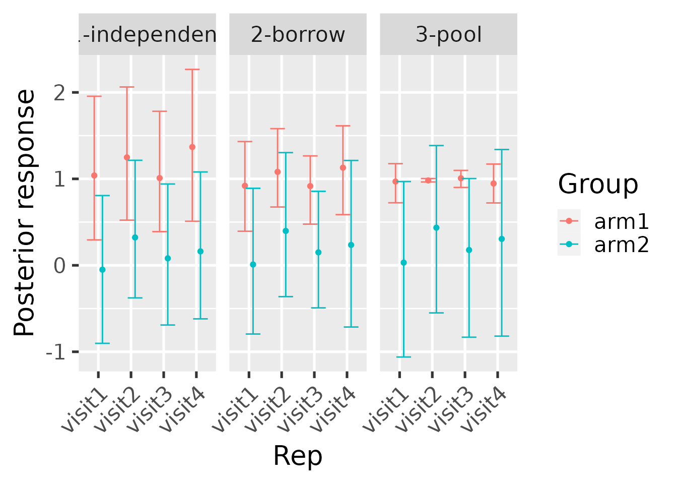
hbl_plot_group() shows the same information but grouped by the group designations in the data (e.g. treatment arm). The results below are not actually correct because the MCMCs ran for so few iterations. For serious analyses, increase the iter and warmup arguments to several thousand and increase the number of chains to about 3 or 4.

hbl_plot_group(
  borrow = summary_hierarchical,
  pool = summary_pool,
  independent = summary_independent
)

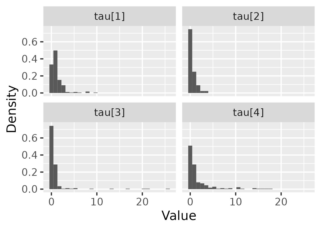
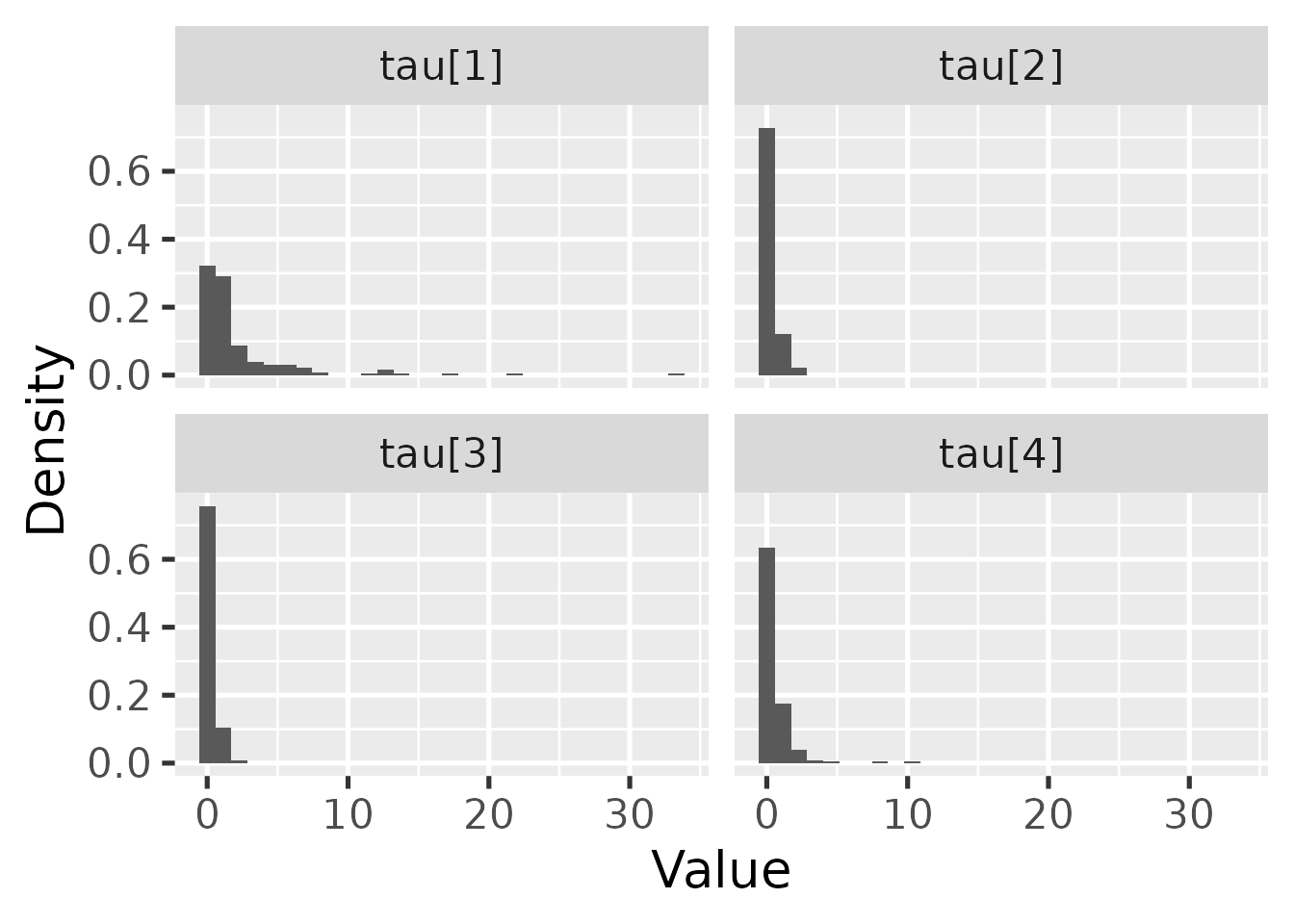
hbl_plot_tau() visualizes the marginal posterior of $\tau$ .

hbl_plot_tau(mcmc_hierarchical)